2021. 7. 9. 21:53ㆍ(Python) Pandas를 이용한 데이터분석
Seaborn은 Matplotlib의 기능과 스타일을 확장한 파이썬 시각화 도구의 고급버전이다.
데이터는 Seaborn 내장 데이터인 titanic 데이터를 사용한다.
처음으로 회귀선이 있는 산점도 그래프를 그려본다.
regplot() 함수는 사로 다른 2개의 연속 변수 사이의 산점도를 그리고 선형 회귀분석에 의한
회귀선을 함께 나타낸다. fit_reg = False 옵션을 설정하면 회귀선을 안보이게 할 수 있다.
import seaborn as sns
import matplotlib.pyplot as plt


plt.style.use('seaborn-poster')
plt.rcParams['axes.unicode_minus'] = False

titanic = sns.load_dataset('titanic')

#스타일 테마 설정(darkgrid, whitegrid, dark, whitem ticks 중에)
sns.set_style('darkgrid')

#그래프 객체 생성(figure에 2개의 서브 플롯 생성)
fig = plt.figure(figsize=(15,5))
ax1 = fig.add_subplot(1,2,1)
ax2 = fig.add_subplot(1,2,2)

#그래프 그리기(선형
sns.regplot(x = 'age',
            y = 'fare',
            data = titanic,
            ax = ax1)

sns.regplot(x = 'age',
            y = 'fare',
            data = titanic,
            ax = ax2,
            color = 'orange',
            fit_reg = False)#회귀선 미표시

plt.show()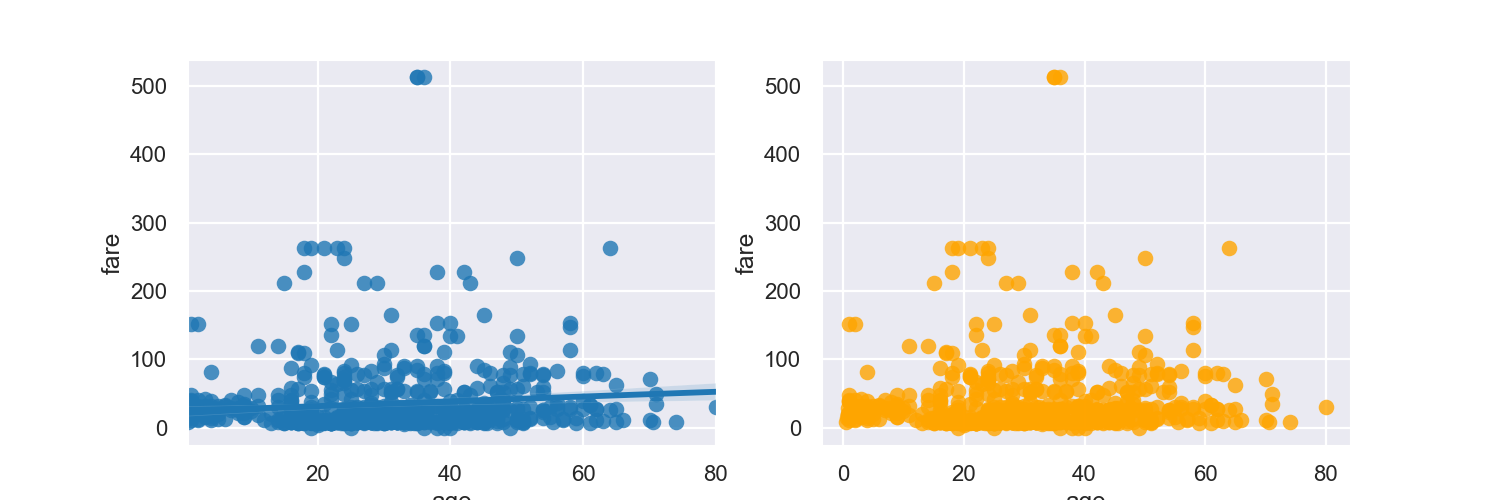
히스토그램/커널 밀도 그래프
단변수( 하나의 변수) 데이터의 분포를 확인할 때 distplot() 함수를 이용한다. 기본값으로 히스토그램과
커널 밀도 함수를 그래프로 출력한다.
distplot = 밀도그래프
histplot = 히스토그램 그래프
import seaborn as sns
import matplotlib.pyplot as plt

plt.rc("font",family = "Malgun Gothic")
sns.set(font = "Malgun Gothic",
        rc = {"axes.unicode_minus":False},
        style = "darkgrid")


plt.style.use('seaborn-poster')
plt.rcParams['axes.unicode_minus'] = False

titanic = sns.load_dataset('titanic')

#스타일 테마 설정(darkgrid, whitegrid, dark, whitem ticks 중에)
# sns.set_style('darkgrid')

fig = plt.figure(figsize=(15,5))
ax1 = fig.add_subplot(1,3,1)
ax2 = fig.add_subplot(1,3,2)
ax3 = fig.add_subplot(1,3,3)

#displot
sns.distplot(titanic['fare'],ax = ax1)

#kdeplot
sns.kdeplot(x = 'fare',data = titanic, ax = ax2)

#histplo
sns.histplot(x = 'fare',data= titanic,ax = ax3)

#차트제목표시

ax1.set_title('titanic fare - hist/ked')
ax2.set_title('titanic fare - kde')
ax3.set_title('titanic fare - hist')

plt.show()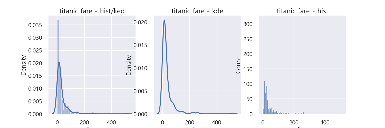
근데 실행은 잘되는데 경고문이 하나뜬다.
FutureWarning: `distplot` is a deprecated function and will be removed in a future version. Please adapt your code to use either `displot` (a figure-level function with similar flexibility) or `histplot` (an axes-level function for histograms).
warnings.warn(msg, FutureWarning)
보니깐 displot 이 미래버젼에는 사라진다는 것이었다.
히트맵
Seaborn 라이브러리는 히트맵을 그리는 heatmap() 함수를 제공한다.
2개의 범주형 변수를 각각 x,y 축에 놓고 데이터를 매트릭스 형태로 분류한다.
데이터프레임을 피벗테이블로 정리할때 한 변수를 행 인덱스로
나머지 변수를 열 이름으로 설정한다.
import seaborn as sns
import matplotlib.pyplot as plt

plt.rc("font",family = "Malgun Gothic")
sns.set(font = "Malgun Gothic",
        rc = {"axes.unicode_minus":False},
        style = "darkgrid")

plt.rcParams['axes.unicode_minus'] = False

titanic = sns.load_dataset('titanic')

table = titanic.pivot_table(index=['sex'],columns=['class'],aggfunc='size')  #aggfunc = 'size' 옵션은 데이터 값의 크기를 기준으로 집계한다는 뜻이다.

#히트맵 그리기
sns.heatmap(table, #데이터프래임
            annot = True, fmt = 'd', #데이터 값 표시여부, 정수형 포맷
            cmap = 'YlGnBu', #컬러 맵
            linewidth = 5, #구분선
            cbar= False) #컬러바 표시여부

plt.show()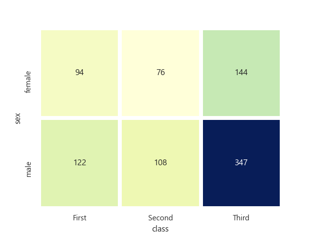
범주형 데이터의 산점도
범주형 변수에 들어 있는 각 볌주별 데이터의 분포를 확인하는 방법이다.
stripplot() 함수와 swarmplot() 함수를 사용할 수 있다.
swarmplot() 함수는 데이터의 분산까지 고려하여, 데이터 포인트가
서로 중복되지 않도록 그린다.
import seaborn as sns
import matplotlib.pyplot as plt

titanic = sns.load_dataset('titanic')

#스타일 테마 설정
sns.set_style('whitegrid')

#그래프 객체 생성

fig = plt.figure(figsize=(15,5))
ax1 = fig.add_subplot(1,2,1)
ax2 = fig.add_subplot(1,2,2)

#이산형 변수의 분포 - 데이터 분산 비고려(중복 표시 O)

sns.stripplot(x = "class",
              y = "age",
              data = titanic,
              ax = ax1)
#이산형 변수의 분포 - 데이터 분산 고려( 중복표시 x)
sns.swarmplot( x= "class",
               y = "age",
               data = titanic,
               ax = ax2)
ax1.set_title('Strip plot')
ax2.set_title('Strip plot')

plt.show()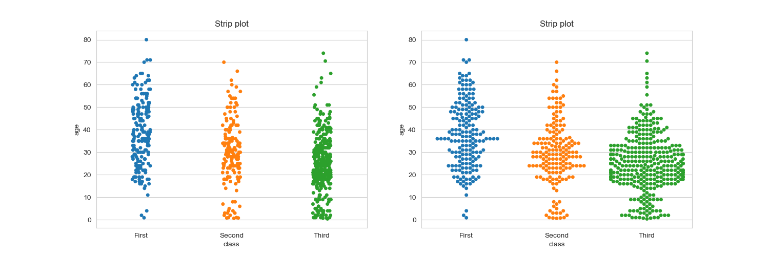
막대그래프
막대그래프는 barplot() 함수로 그리고 3개의 axe 객체 (서브플롯) 을 만들고, 옵션에 변화를 주면서
차이를 살펴보자. x축 y축에 변수 할당 , x축 y축에 변수 할당하고 hue옵션 추가 x축 y축에 변수 할당하고
hue옵션을 추가하여 누적출력 순으로 실행한다.
hue옵션에 class변수를 추가하면 sex변수안에서 class가 어떻게 나뉘는지 세부적으로 볼수있다.
import seaborn as sns
import matplotlib.pyplot as plt

titanic = sns.load_dataset('titanic')

#스타일 테마 설정
sns.set_style('whitegrid')

#그래프 객체 생성
fig = plt.figure(figsize=(15,5))
ax1 = fig.add_subplot(1,3,1)
ax2 = fig.add_subplot(1,3,2)
ax3 = fig.add_subplot(1,3,3)

#x축 y축에 변수 할당
sns.barplot(x = 'sex',y = 'age', data = titanic ,ax =ax1)

# x축 y축에 변수 할당하고 hue 옵션을 추가한다
#hue 여러열에서 집단묶어서 세부 집단 시각화
sns.barplot(x = 'sex', y = 'age', data = titanic, hue = 'class',ax = ax2)

# x축 y축에 변수 할당하고 hue옵션을 추가하여 누적출력
sns.barplot(x = 'sex', y = 'age', data = titanic , hue = 'class', dodge = False ,ax = ax3)

ax1.set_title('titanic survived - sex')
ax2.set_title('titanic survived - sex/class')
ax3.set_title('titanic survived - sex/class(stacked)')

plt.show()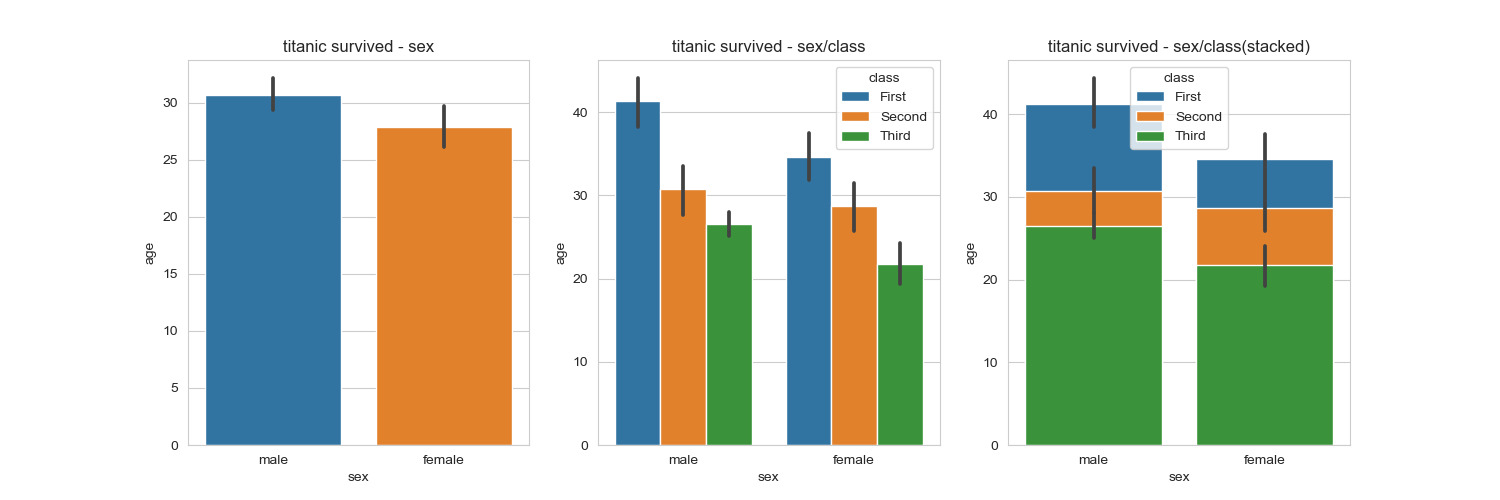
빈도그래프
각 범주에 속하는 데이터의 개수를 막대 그래프로 나타내는 countplot() 함수를 사용해보자.
3개의 서브플롯을 비교한다. 기본설정, hue 옵션 추가, 축방향으로 hue 변수를 분리하지 않고
위로 쌓아 올리는 누적 그래프로 출력 3개를 비교해보자.
import seaborn as sns
import matplotlib.pyplot as plt

titanic = sns.load_dataset('titanic')

#스타일 테마 설정
sns.set_style('whitegrid')

#그래프 객체 생성
fig = plt.figure(figsize=(15,5))
ax1 = fig.add_subplot(1,3,1)
ax2 = fig.add_subplot(1,3,2)
ax3 = fig.add_subplot(1,3,3)

#기본값
sns.countplot(x = 'class',palette = 'Set1',data = titanic, ax =ax1)

#hue 옵션에 who 추가
sns.countplot(x = 'class',hue = 'who',palette = 'Set2',data= titanic, ax = ax2)

#dodge = False 옵션 추가 (축 방향으로 분리하지 않고 누적 그래프 출력)
sns.countplot(x = 'class',hue = 'who',palette = 'Set3',data= titanic, dodge = False,ax = ax3)

ax1.set_title('titanic class')
ax2.set_title('titanic class - who')
ax3.set_title('titanic class - who(stacked)')

plt.show()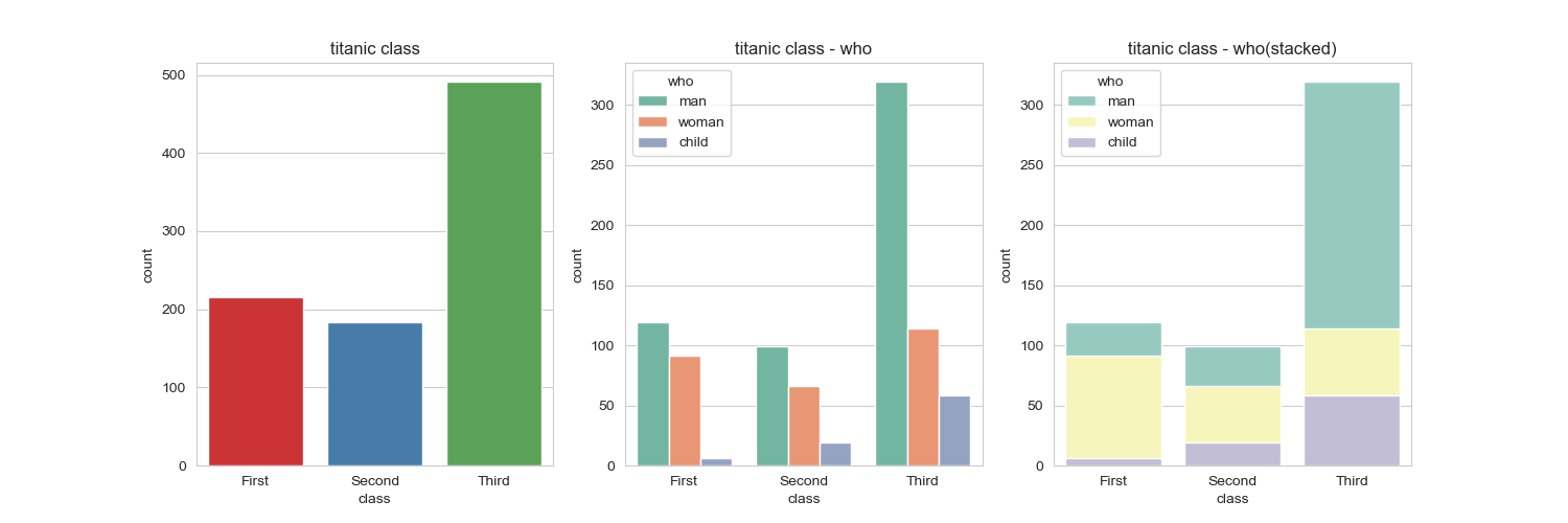
박스플롯/ 바이올린 그래프
박스플롯은 범주형 데이터 분포와 주요 통계 지표를 함께 제공한다. 다만 박스 플롯 만으로는
데이터가 퍼져있는 분산의 정도를 정확하게 알기는 어렵기 때문에 커널 밀도 함수 그래프를
y축 방향에 추가하여 바이올린 그래프를 그리는 경우도 있다.
boxplot() 함수로 박스플롯 그래프를 그리고 , violinplot() 함수를 통해 바이올린 그래프를 그린다.
hue 변수에 sex를 추가 하면 남녀 데이터를 구분하여 표시할수 있다.
import matplotlib.pyplot as plt
import seaborn as sns

titanic = sns.load_dataset('titanic')

sns.set_style('whitegrid')

#그래프 객체 생성
fig = plt.figure(figsize=(15,10))
ax1 = fig.add_subplot(2,2,1)
ax2 = fig.add_subplot(2,2,2)
ax3 = fig.add_subplot(2,2,3)
ax4 = fig.add_subplot(2,2,4)

#박스플롯
sns.boxplot(x = 'alive', y = 'age', data = titanic, ax = ax1)

#박스플롯 그래프 -hue 변수추가
sns.boxplot(x = 'alive',y = 'age',hue = 'sex', data = titanic, ax =ax2)

#바이올린 그래프
sns.violinplot(x = 'alive', y= 'age',data = titanic, ax = ax3)

#바이올린 그래프 - hue 변수추가
sns.violinplot(x = 'alive', y = 'age',hue = 'sex', data = titanic , ax = ax4)

plt.show()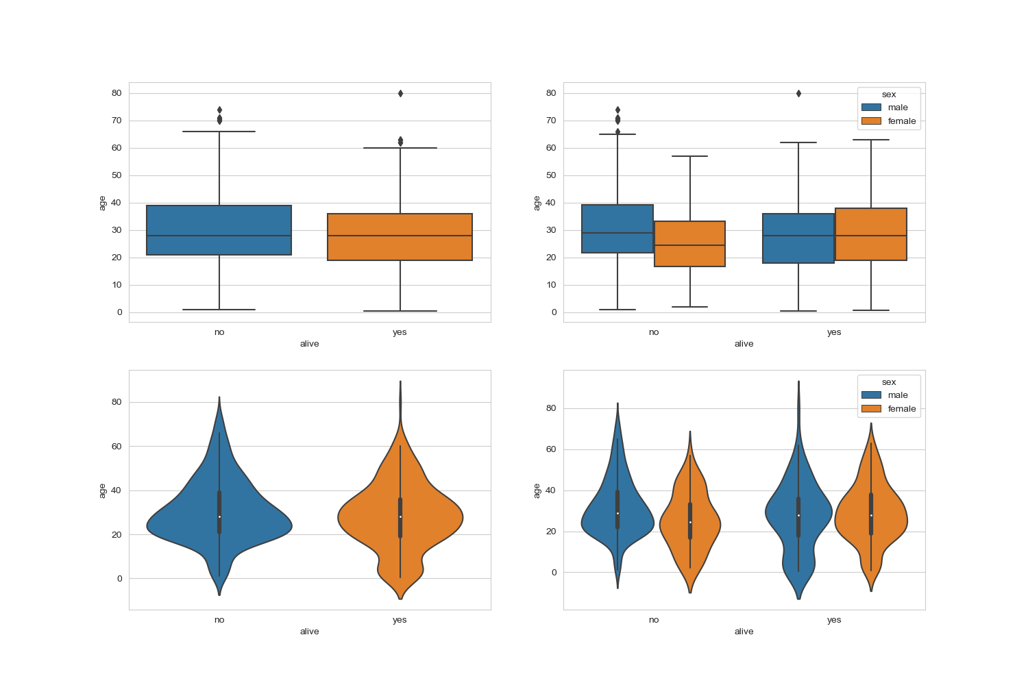
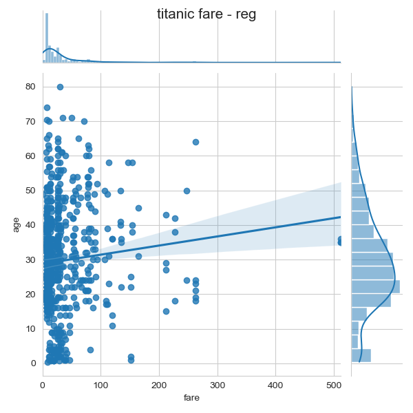
조인트 그래프
jointplot() 함수는 산점도를 기본으로 표시하고, x-y 축에 각 변수에 대한 히스토그램을 동시에 보여준다.
따라서 두 변수의 관계와 데이터가 분산되어 있는 정도를 한눈에 파악하기 좋다.
밑에서 해볼건 산점도,회귀선추가,육각산점도,커널밀집그래프 순으로 조인트그래프를 그려본다.
import matplotlib.pyplot as plt
import seaborn as sns
titanic = sns.load_dataset('titanic')
sns.set_style('whitegrid')
#조인트 그래프 -산점도
j1 = sns.jointplot(x = 'fare',y = 'age', data =titanic)
#조인트 그래프 - 회귀선
j2 = sns.jointplot(x = 'fare', y = 'age',kind = 'reg',data = titanic)
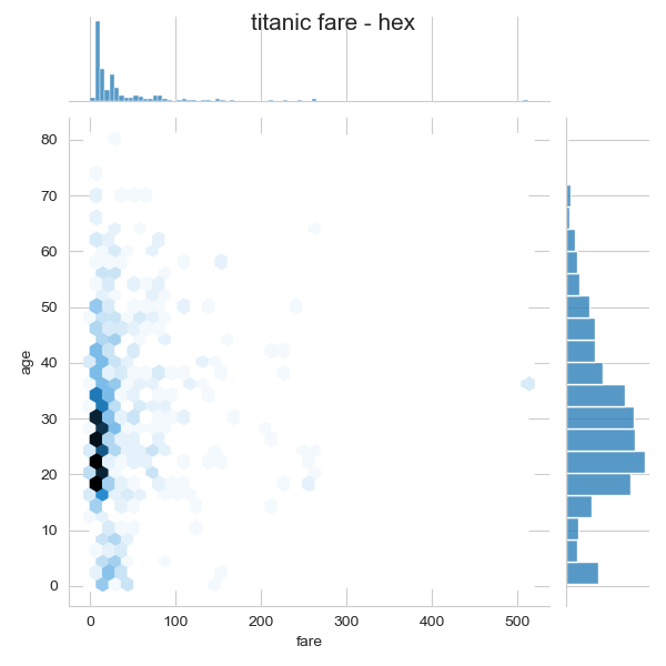
#조인트 그래프 - 육각 그래프
j3 = sns.jointplot(x = 'fare', y = 'age', kind = 'hex', data =titanic)
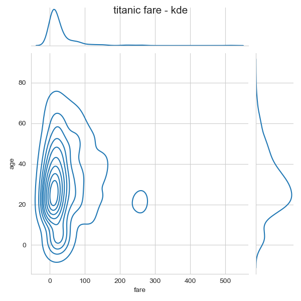
#조인트 그래프 - 커널 밀집 그래프
j4 = sns.jointplot(x = 'fare' , y= 'age', kind = 'kde', data = titanic)
j1.fig.suptitle('titanic fare - scatter', size = 15)
j2.fig.suptitle('titanic fare - reg',size = 15)
j3.fig.suptitle('titanic fare - hex',size =15)
j4.fig.suptitle('titanic fare - kde',size= 15)
plt.show()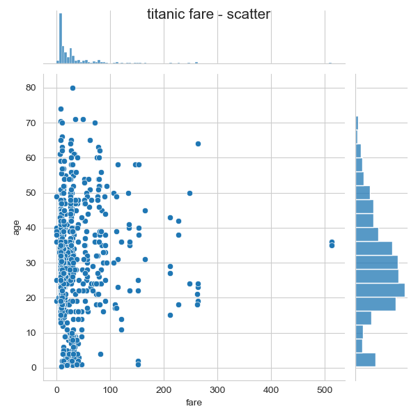
조건을 적용하여 화면을 그리드로 분할하기
FacetGrid() 함수는 행,열 방향으로 서로 다른 조건을 적용하여 여러개의 서브플롯을 만든다.
그리고 각 서브 플롯에 적용할 그래프 종류를 map() 메소드를 이용하여 그리드 객체에 전달한다.
밑의 코드에서는 열 방향으로는 who 열의 탑승객 구분(man, woman , child) 값으로 구분하고
행 방향으로는 survived 열의 구조 ( 1 = 구조, 0 = 구조실패) 값으로 구분하여 2X3 모양의 그리드를 만든다.
import matplotlib.pyplot as plt
import seaborn as sns

titanic =sns.load_dataset('titanic')

sns.set_style('whitegrid')

#조건에 따라 그리드 나누기
g = sns.FacetGrid(data = titanic,col = 'who', row = 'survived')

#그래프 적용하기
g = g.map(plt.hist,'age')
plt.show()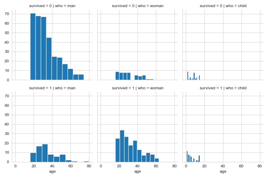
여기서 pairplot() 함수를 이용, 잔달되는 데이터프레임의 짝을 지을수 있다.
titanic_pair = titanic[['age','pclass','fare']]

g = sns.pairplot(titanic_pair)
plt.show()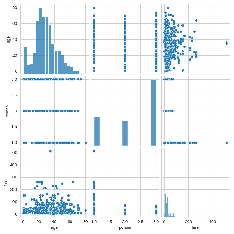
'(Python) Pandas를 이용한 데이터분석' 카테고리의 다른 글
| 데이터전처리 (0) | 2021.07.15 |
|---|---|
| Folium 라이브러리를 이용한 지도 표현 (0) | 2021.07.09 |
| 여러가지 시각화 그래프(Histogram & Scatter & Pie Chart & Box Plot) (0) | 2021.07.09 |
| Matplotlib 을 통한 인구 이동 그래프(2) (0) | 2021.07.08 |
| Matplotlib 을 통한 인구 이동 그래프(1) (0) | 2021.07.08 |