2021. 6. 24. 11:43ㆍR 공부/지도학습
선형 회귀 분석과 다른점
선형 회귀 분석의 종속변수(타겟)은 범위가 무제한으로 모든값을 가질수 있다.
그리고 종속변수는 숫자(연속) 여야 가능하다.
로지스틱 회귀분석은 종속 변수값의 제한이 있다. 가능한 범위가 있고 가질수없는 값이 존재한다.
종속변수는 범주형이며 연속이어도 되지만, 숫자일려면 범위가 확실하게 정해져 있어야한다.
종속변수가 0과 1사이의 값일때 우리는 분류 또는 예측을 할수있다.
분류는 0또는 1 , 예측은 1일 확률 이런식으로 나온다.
선형 회귀분석(z값이 -부터 + 까지 어느값이던 가능하다.)

로지스틱 회귀분석을 위해 식을 바꿨다.
그러면 y값이 0에서 1로 제한된다.

하지만 y만 보면 무슨 문자인지 알수없다. 그래서 y를 바꿔준다.

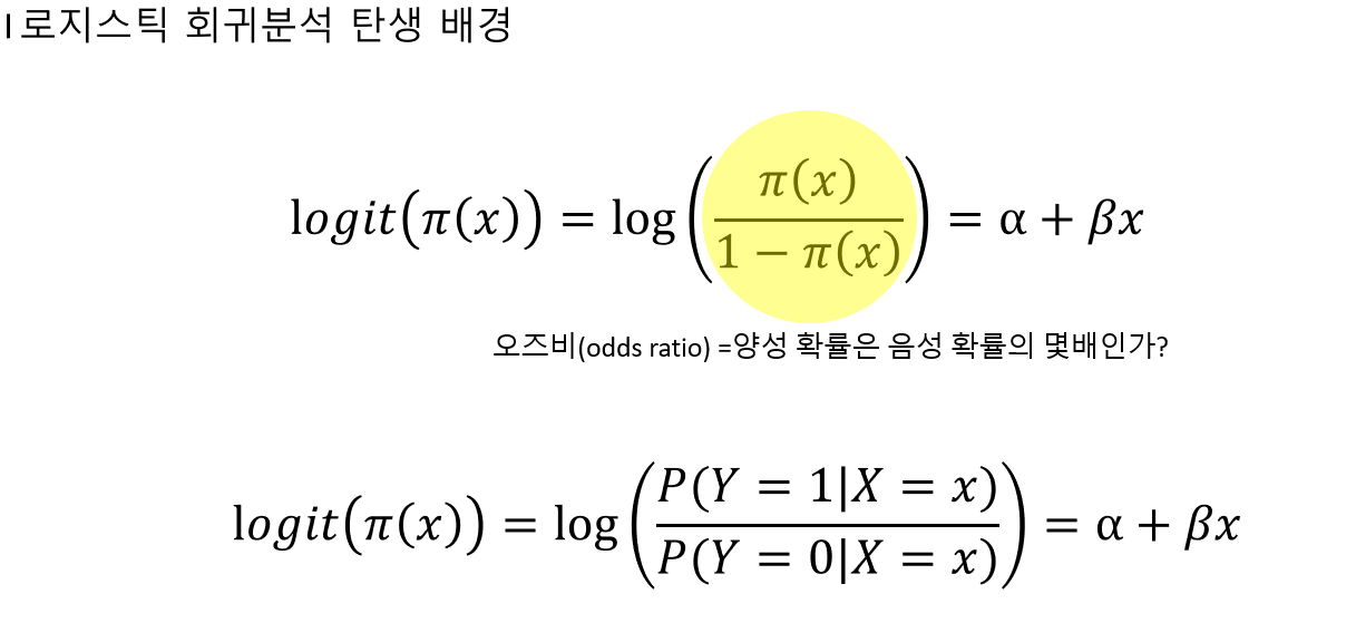
파이x는 Y =1 일때 확률이고 1-파이x는 1에서 Y=1일때 확률을 뺀거니까 Y=0일 확률이다.
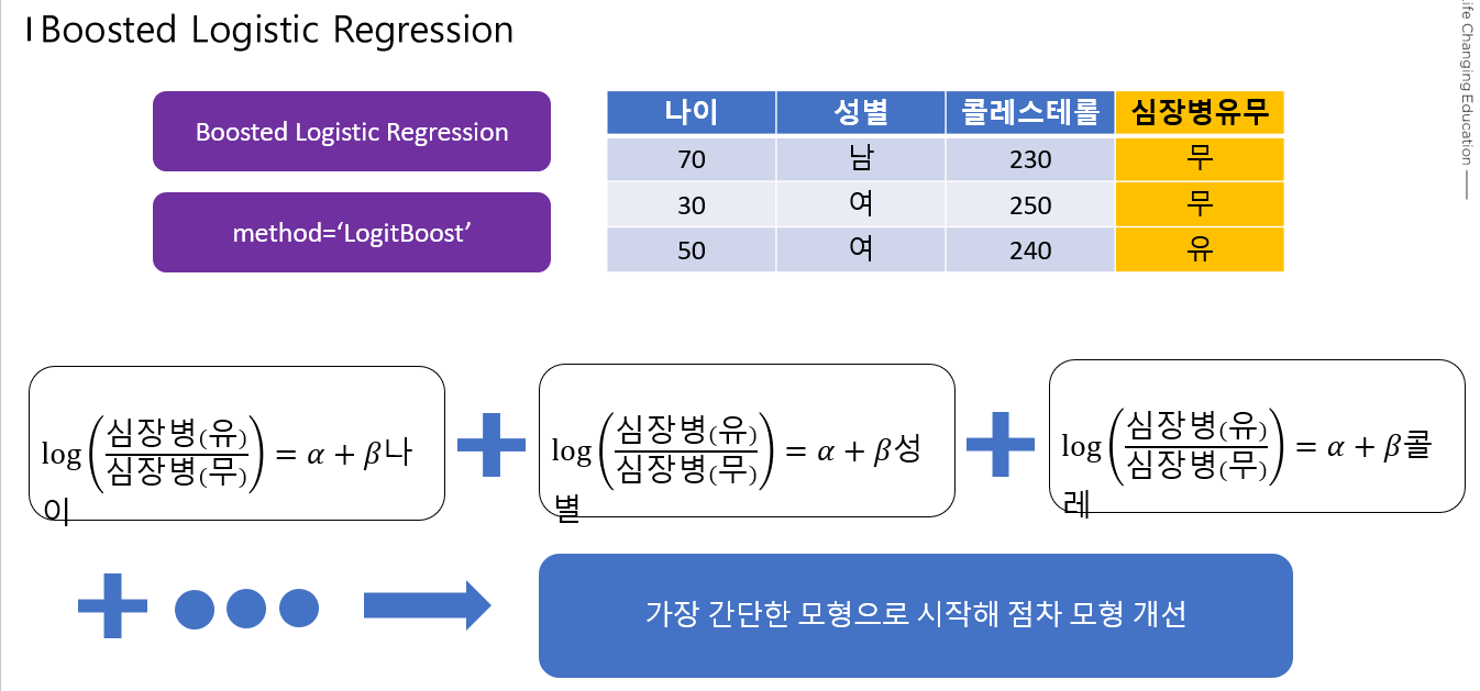
일단 로지스틱 회귀분석 모형에 4가지 정도가 있다

Boosted : 약한것을 계속 더해가면서 강하게 만듬
Logistic Model Trees: 로지스틱+트리 개념
Penalized: 페널티를 준다.
Regularized : Penalized 랑 비슷
Boosted
Logistic Model Trees

Penalized

베타 영역에 제한을 준다(페널티를준다)
Regularized

이제 실제 코드로 알아보자
오늘 사용할 데이터는 심장병 유무에 대한 데이터 이다.
타겟 데이터는 심장병의 유무의 변수다.

rawdata$target <- as.factor(rawdata$target)
unique(rawdata$target) #결과확인, 유일한 값들을 보여줌 0,1,0,0,1 와 같이 여러숫자가 있을때 0,1만보여줌
[1] 1 0
Levels: 0
그리고 연속형 독립변수 표준화를 해준다
rawdata$age <- scale(rawdata$age)
rawdata$trestbps <- scale(rawdata$trestbps)
rawdata$chol <- scale(rawdata$chol)
rawdata$thalach <- scale(rawdata$thalach)
rawdata$oldpeak <- scale(rawdata$oldpeak)
rawdata$slope <- scale(rawdata$slope)
그다음 범주형 독립변수 는 as.factor를 해준다.
newdata <- rawdata

factorVar <- c("sex","cp","fbs","restecg","exang","ca")
newdata[,factorVar] = lapply(newdata[,factorVar],factor)
그리고 데이터를 트레이닝, 테스트 셋으로 나눈다.
#트레이닝 테스트 나누기(7:3)
set.seed(2020)
datatotal <- sort(sample(nrow(newdata),nrow(newdata)*0.7))
train <- newdata[datatotal,]
test <- newdata[-datatotal,]

train_x <- train[,1:12]
train_y <- train[,13]

test_x <- test[,1:12]
test_y <- test[,13]
그리고 트레이닝 시켜보자
#LogitBoost
ctrl <- trainControl(method = "repeatedcv",repeats = 5)
logitFit <- train(target~.,
data = train,
method = "LogitBoost",
trControl = ctrl,
metric = "Accuracy"
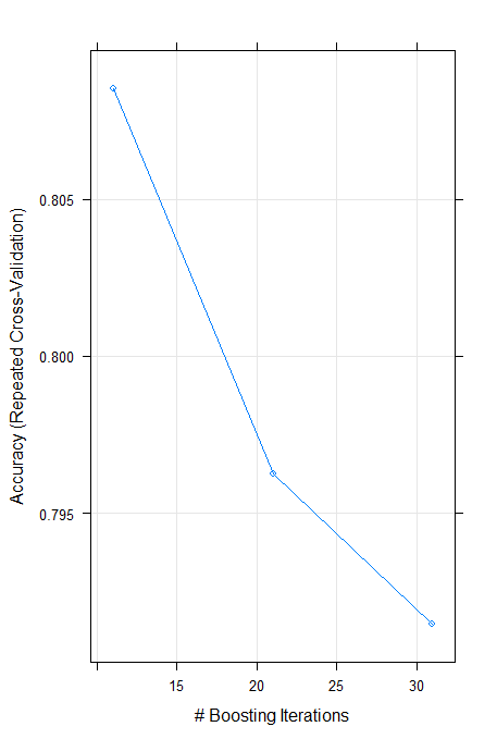
)결과를 보면
logitFIt

Boosted Logistic Regression

212 samples
 13 predictor
  2 classes: '0', '1'

No pre-processing
Resampling: Cross-Validated (10 fold, repeated 5 times)
Summary of sample sizes: 191, 190, 191, 191, 191, 191, ...
Resampling results across tuning parameters:

  nIter  Accuracy   Kappa
  11     0.8085281  0.6049673
  21     0.7962771  0.5823803
  31     0.7914719  0.5729374

Accuracy was used to select the optimal model using
 the largest value.
The final value used for the model was nIter = 11.
약한것들이 여러번 반복된다.
가장 정확할때는 11번을 학습했을때이다.
결과를 예측해보면
pre_test <- predict(logitFit,newdata = test)
confusionMatrix(pre_test,test$target)


Confusion Matrix and Statistics

          Reference
Prediction  0  1
         0 36  8
         1 12 35

               Accuracy : 0.7802
                 95% CI : (0.6812, 0.8603)
    No Information Rate : 0.5275
    P-Value [Acc > NIR] : 5.446e-07

                  Kappa : 0.5612

 Mcnemar's Test P-Value : 0.5023

            Sensitivity : 0.7500
            Specificity : 0.8140
         Pos Pred Value : 0.8182
         Neg Pred Value : 0.7447
             Prevalence : 0.5275
         Detection Rate : 0.3956
   Detection Prevalence : 0.4835
      Balanced Accuracy : 0.7820

       'Positive' Class : 0
정확도가 78%정도로 나온다.
그리고 가장 중요한 변수를 보면
importance_logit <- varImp(logitFit,scale = FALSE)
plot(importance_logit)

cp가 1등이다.
'R 공부 > 지도학습' 카테고리의 다른 글
| Decision Tree 와 Random_Forest (0) | 2021.06.25 |
|---|---|
| Naive Bayes Classification (0) | 2021.06.24 |
| KNN(K-Nearest Neighbor) (2) | 2021.06.23 |